Memory Down

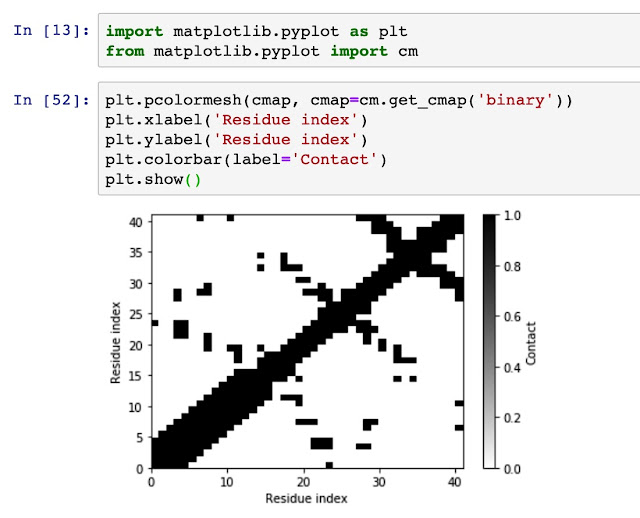
Generate residue-residue contact matrix for MD simulation trajectories Using residue-residue contact map to understand the distance and spatial relationship is important for protein dynamics and protein 3D conformation modeling. Here in this tutorial, I use mdtraj to demonstrate how to generate a contact map from a static single-frame PDB file and visualise it with matplotlib. Taken mini protein gHEEE_02 as an example, we first load the pdb file (generated from rosetta modeling). You could virtually take any protein containing PDB file as an example, such as 5W9F. # load mdtraj package  import mdtraj as mt # load the pdb file and transform it into a mdtraj.Trajectory object p = mt.load_pdb("5W9F.pdb") # now we could check some properties of the trajectory object p <mdtraj.Trajectory with 1 frames, 335 atoms, 41 residues, without unitcells at 0x820a38208> Therefore, we know that this protein contains 1 frame, 41 residues.

Protein-ligand binding prediction with machine learning models: current status Drug discovery is a long journey. Given the complexity of a new drug design project, only through the highly organized cooperations between different people, the goal of developing a new drug could be achieved. In the whole process, the binding affinity prediction between a target (a protein in general) and a small compound would be useful before the cell model or animal model experiments. We hope to discover tightly bound small molecules to a specific protein. Improving the bind affinity prediction could help us short list a set of useful molecules (lead-like compounds). Traditionally, binding affinity prediction could be achieved by absolute binding energy calculation, MMGBSA and scoring functions (in virtual screening and docking). More and more machine learning based methods have been developed to perform the prediction (Table 1). Table 1. Current ML-based binding affinity prediction models

A step-by-step tutorial to perform PCA with Gromacs MD trajectory It is a common practice to perform principal component analysis to explore the transitions and dynamics of macromolecules simulations.   There may exist multiple states in the free energy landscape, so it is important to extract the representative structures from the energy minima in the free energy surface. To generate such a free energy surface, we could define some collective variables (CVs). However, due to the high dimensionality of the simulation trajectory, it is not always straightforward to select several more important CVs. So the problem is how could we find one or two CVs which could describe the slow motions of the system? To this end, PCA-based dimension reduction and projections could partially solve the problem by transforming the original dataset and grasp the largest variance of the system. Although there has been a tool in Gromacs, which perform the PCA using g_covar and g_anaeig. Th