Fixing bugs in FF14SB port for Gromacs

Generate residue-residue contact matrix for MD simulation trajectories

Using residue-residue contact map to understand the distance and spatial relationship is important for protein dynamics and protein 3D conformation modeling.

Here in this tutorial, I use mdtraj to demonstrate how to generate a contact map from a static single-frame PDB file and visualise it with matplotlib. Taken mini protein gHEEE_02 as an example, we first load the pdb file (generated from rosetta modeling). You could virtually take any protein containing PDB file as an example, such as 5W9F.

# load mdtraj package 

import mdtraj as mt

# load the pdb file and transform it into a mdtraj.Trajectory object

p = mt.load_pdb("5W9F.pdb")

# now we could check some properties of the trajectory object

p

<mdtraj.Trajectory with 1 frames, 335 atoms, 41 residues, without unitcells at 0x820a38208>

Therefore, we know that this protein contains 1 frame, 41 residues. For each residue, we could calculate the distance between it with all other residues only considering the alpha Carbon distance. After calculation, we should be able to obtain a 41X41 matrix, where each bin contains one distance between residue i and j. 

# we first get the atom indices of each one of the 41 residues

indices = p.topology.select("name CA")

# then we create an atom-pair list, with 41*41 residue-residue combinations

import itertoolspairs =list( itertools.product(pairs, pairs))

# now we calcuate the distances for all 41*41 pairs of atoms. 

distmtx = mt.compute_distances(p, atom_pairs=pairs)

Next, we determine whether a pair of residues has a contact by comparing the distance between them with a cutoff, 0.8 nm, which is a common practice. Remember, the distance matrix calculated from mdtraj uses the "nanometer" as the unit. 

# now we reshape the one-dimensional 41*41 length array into a matrix with shape = 41X41

distmtx = distmtx.reshape((41, 41))

# we get the contact matrix from the distance matrix

cmap = ( distmtx <= 0.8) * 1.0

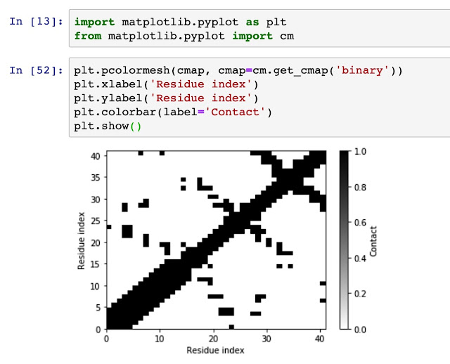
Now, we use matplotlib to visulize the contact matrix.

import matplotlib.pyplot as plt

from matplotlib.pyplot import cm

# plot

plt.pcolormesh(cmap, cmap=cm.get_cmap('binary'))

# add labels

plt.xlabel('Residue index')

plt.ylabel('Residue index')

# add colorbar

plt.colorbar(label='Contact')

plt.show()

Now we have already generate a contact map for a pdb file, we will generate a contact probability map for a trajectory file. To be continued.